Getting Started with RyouSick • RyouSick

Simulation

To illustrate the use of the RyouSick package, lets go through an example, where we simulate a disease called bad-knee syndrome in a population.

Before simulating genotypes and case-control phenotype data using RyouSick, we first need to simulate the disease parameters with the function sim_disease(). The disease parameters for our target disorder is simulated on 10 SNPs with a heritability $h^2$ of 0.8 and a prevalence in the population of 0.25:

library("RyouSick")
bad_knee_syndrome <- sim_disease(n_snp = 10, h2 = 0.8, prevalence = 0.25)

Output disease parameters:

bad_knee_syndrome
#> $MAF
#>  [1] 0.40071281 0.22309419 0.04419435 0.42861384 0.46978992 0.15051858
#>  [7] 0.15620303 0.11896250 0.07729138 0.20345860
#> 
#> $BETA
#>  [1]  0.000000  0.000000  0.000000 -0.296382  0.000000  0.000000  0.000000
#>  [8]  0.000000  0.000000  0.000000
#> 
#> $CAUSAL
#>  [1] 0 0 0 1 0 0 0 0 0 0
#> 
#> $H2
#> [1] 0.8
#> 
#> $PREVALENCE
#> [1] 0.25
#> 
#> $N_SNP
#> [1] 10

In the above output, each MAF value at a given index indicates the frequency at which the genome will vary from the reference genome. The CAUSAL vector and BETA vector likewise tell us which SNPs are simulated to be causally connected to developing the simulated disease and how big of an effect they have. In the above output we can see that SNP 4 has been simulated to be causal.

We can now chose what kind of simulation we want to perform for our population. Either with family history or without using one of the two functions:

sim_genotypes_no_family() simulates genotype and case-control phenotype without family case-control phenotypes
sim_genotypes_with_family() simulates genotype and case-control phenotype with family case-control phenotypes

Lets try to simulate 10 genotypes/individuals with the simulation sim_genotypes_with_family(), with the bad_knee_syndrome disease parameters, and with 1 to 3 siblings for each individual and save it under the filename “bad_knee_data10x10”:

bad_knee_data <- sim_genotypes_with_family(n = 10, 
                                           disease = bad_knee_syndrome, 
                                           path = "bad_knee_data10x10", 
                                           n_sibs = c(1,2,3))

The bad_knee_data will now contain a list object, which we will refer to as an rds object, with a reference to a file-backed matrix (matrix stored on disk), a tibble containing information on SNPs (MAP) and a tibble containing phenotype information on the genotypes (FAM). Individual columns in the data can be accessed using the dollar notation.

bad_knee_data$FAM$Status
#>       [,1]
#>  [1,]    1
#>  [2,]    0
#>  [3,]    0
#>  [4,]    0
#>  [5,]    0
#>  [6,]    1
#>  [7,]    0
#>  [8,]    0
#>  [9,]    1
#> [10,]    0

Slices of the genotype data can be accessed as well.

bad_knee_data$genotypes[1:10, 1:10]
#>       [,1] [,2] [,3] [,4] [,5] [,6] [,7] [,8] [,9] [,10]
#>  [1,]    0    2    0    0    0    0    0    0    0     1
#>  [2,]    1    0    1    2    0    0    0    1    0     1
#>  [3,]    0    0    0    1    1    0    0    1    1     1
#>  [4,]    0    1    0    0    1    0    0    1    0     0
#>  [5,]    0    1    0    0    0    0    0    1    0     0
#>  [6,]    0    0    0    0    0    1    1    0    0     1
#>  [7,]    1    1    0    2    1    1    1    0    0     1
#>  [8,]    0    0    0    2    1    0    0    0    0     0
#>  [9,]    0    0    0    0    0    0    0    1    0     1
#> [10,]    0    0    0    2    1    0    0    0    0     0

Here each row represents an individual’s genotype and each column a SNP. (WARNING: we highly advise against indexing all the data at once using [ ], as this will try to load the whole file-backed matrix into memory, which, depending on the size of the file, might cause problems)

All of the simulated information contained in our example case bad_knee_data can be seen below.

knitr::kable(bad_knee_data$MAP, align = "ccc")

SNP_ID	MAF	BETA
1	0.4007128	0.000000
2	0.2230942	0.000000
3	0.0441943	0.000000
4	0.4286138	-0.296382
5	0.4697899	0.000000
6	0.1505186	0.000000
7	0.1562030	0.000000
8	0.1189625	0.000000
9	0.0772914	0.000000
10	0.2034586	0.000000

knitr::kable(bad_knee_data$FAM, align = "ccccccc")

ID	Genetic_Liability	Full_Liability	Status	p1_Status	sibs_Status
1	0.36302377	1.0514806	1	0	1
2	-0.48394788	-1.2211161	0	0	0, 0, 0
3	-0.06046206	0.2717148	0	0	0, 0
4	0.36302377	0.6714890	0	0	1
5	0.36302377	-0.2015389	0	0	0, 1
6	0.36302377	0.7119287	1	1	0, 1, 1
7	-0.48394788	-0.6437396	0	0	0, 0, 0
8	-0.48394788	-0.3891188	0	0	0
9	0.36302377	1.3064947	1	0	0, 0
10	-0.48394788	-0.2376695	0	0	0, 1, 1

Analysis

We now perform analysis on our simulated data. The RyouSick package contains three methods for analyzing the data:

GWAS() Linear regression using genotype data and case-control status
GWAX() Linear regression using genotype data and proxy case-control status
LTFH() Linear regression using genotype data and posterior mean genetic liabilities

Lets now try each of the methods on our data:

x <- GWAS(rds.obj = bad_knee_data, y = bad_knee_data$FAM$Status)
y <- GWAX(rds.obj = bad_knee_data)
z <- LTFH(rds.obj = bad_knee_data, h2 = 0.8, prevalence = 0.25)

The output will consist of estimated effect sizes, standard errors, t-scores and p-values for each SNP, which again can be accessed using dollar notation.

knitr::kable(x)

estim	std.err	score	p.value
-0.3750000	0.3827328	-0.9797959	0.3558838
0.1111111	0.2383068	0.4662524	0.6534672
-0.3333333	0.5270463	-0.6324555	0.5447373
-0.3033708	0.1341274	-2.2618111	0.0535707
-0.6000000	0.2449490	-2.4494897	0.0399685
0.2500000	0.3952847	0.6324555	0.5447373
0.2500000	0.3952847	0.6324555	0.5447373
-0.2000000	0.3162278	-0.6324555	0.5447373
-0.3333333	0.5270463	-0.6324555	0.5447373
0.5000000	0.2795085	1.7888544	0.1114343

Note that to access the analysis data for GWAX and LTFH you have to use method_result$GWAS_Data.

Statistics for the data can be calculated by passing the p-values, the true causal SNPs and a chosen significance level to the get_stats() function

gwas_stats <- get_stats(pvalues = x$p.value, 
                        true_causal = bad_knee_syndrome$CAUSAL, 
                        a = 0.05)
knitr::kable(gwas_stats)

	false_negatives	true_negatives	false_positives	true_positives	total
Count	1.0	8.0	1.0	0	10
Frequency	0.1	0.8	0.1	0	1

Visualizations

We can then visualize the data using the function Manhattan_plot() to get a picture of which SNPs are causal and where in the genome they have been found:

Manhattan_plot(x, a = 5e-7)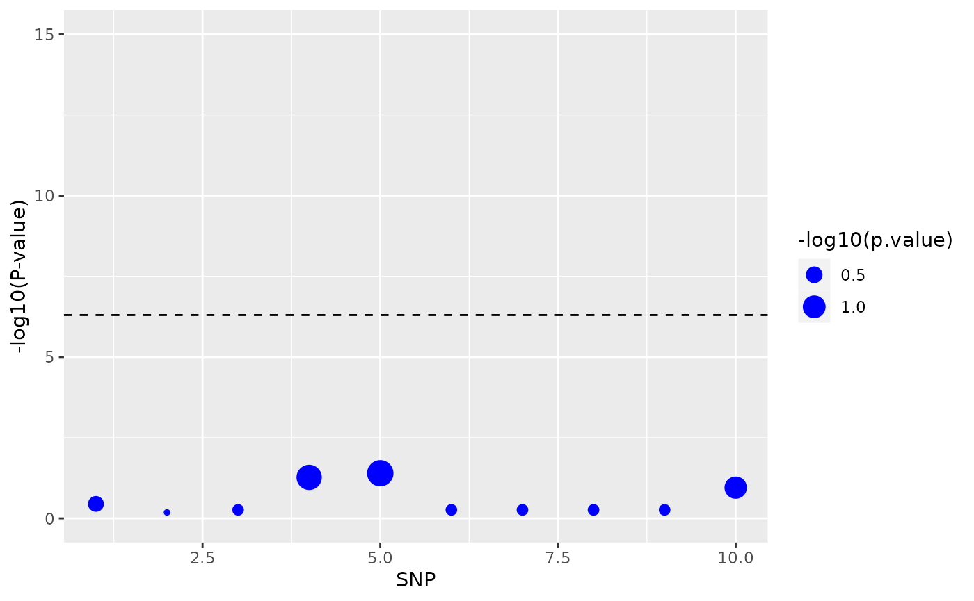

When checking our analysis results we basically want to see which method finds the most causal SNPs, and that the SNPs are actually predetermined to be causal. The function get_stats() will tell us about the frequency of false positives, true positives, false negatives and true negatives for each method, but if we want to visually compare the accumulated power for each of the methods, we can use the function Power_plots().

Before we use the function Power_plots() we need to save the GWAS_data for each method in list format. For illustrative purposes we set the significance level to 0.5.

power_plot_data = list(x, y$GWAS_Data, z$GWAS_Data)

With the data saved, we can now use Power_plots():

Power_plots(Gwas_data = power_plot_data, a = 0.5)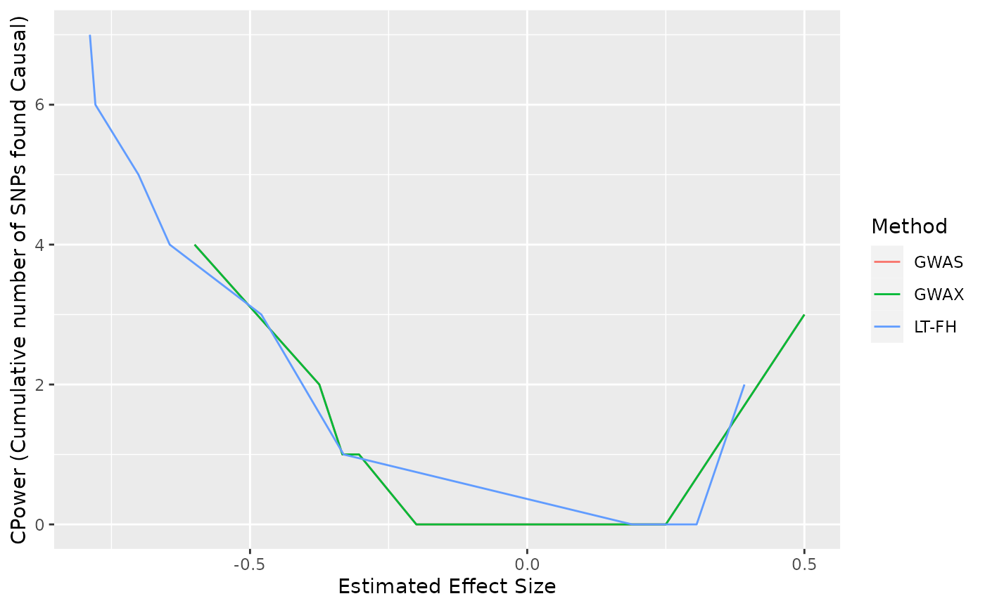

For the output from Power_plots() we note that the line for GWAS cannot be seen in the above plot because it lays under the plot for GWAX, which, when using such a low sample size, produces almost identical results to GWAS.

The x axis of the power plots are estimated effect sizes, which are correlated with the p-value for each SNP. A larger numerical estimated effect size for a SNP, will therefore result in a greater chance of the methods analyzing the SNP to be causal. The y axis is the cumulative number of SNP´s found causal by the methods.

Prediction

As seen in vignette("LTFH") the best method for evaluating causal SNPs is LT-FH. So let’s try to use Prediction_cross_validation() on our LT-FH data to get a model that can predict future cases.

model_results <- Prediction_cross_validation(rds.obj = bad_knee_data,
                                             k = 2,
                                             method = "LTFH")

This model can now be used in the Predict_status() function to predict status for future genotypes. For illustrative purposes we will use our old data again, as the input needs to be formatted as an rds object.

predicted_status <- Predict_status(rds.obj = bad_knee_data,
                                   model = model_results$Best_Model,
                                   prevalence = 0.25)

This gives us the following results.

predicted_status
#>  [1] 1 0 0 0 0 1 0 0 0 0

Compared with the true statuses.

as.vector(bad_knee_data$FAM$Status)
#>  [1] 1 0 0 0 0 1 0 0 1 0

Correct formatting of rds object

If you wish to run the analysis methods on your own data, it must first be formatted properly. To do so, you must first initialize an empty rds file and object matching the size of your data using the createRds() function.

user_input_obj <- createRds("user_input_data", nrow = 10, ncol = 10)

The rds object that is returned can then be filled up by adding columns/vectors in the MAP and FAM tibbles using dollar notation. To integrate with the methods in the package, columns must be given specific names based on their contents. The required information to run must functions and their naming is listed below:

MAF (in MAP): vector with minor allele frequencies for SNPs
Status (in FAM): vector with status for genotypes
p1_Status (in FAM): vector with parent 1 status for genotypes (only used in GWAX and LTFH)
p2_Status (in FAM): vector with parent 2 status for genotypes (only used in GWAX and LTFH)
sibs_Status (in FAM): list containing a vector with sibling status for each genotype or NULL if no siblings for genotype (only used in LTFH)

Note that the names are case-sensitive. An example of filling up the genotypes with a matrix consisting of only 1’s and creating a Status column can be seen below. Remember that when making changes to the tibbles FAM and MAP, the changes to the rds object must be saved using saveRds().

user_input_obj$genotypes[1:10,1:10] <- matrix(1, ncol = 10, nrow = 10)
user_input_obj$Status <- c(1,1,1,0,0,0,0,1,0,0)
saveRds(user_input_obj)

Additionally, it is recommended that the file-backed matrix be filled in blocks if working with large quantities of data (read more in article vignette("Writing_efficient_R_code_and_working_with_large_datasets")). The rds file can later be opened again using the OpenRds() function.

Parallelization

Since most users work on very different computers with various setups, parallelization is not enabled by default. To run simulations using parallelization, which is recommended as it provides a significant speedup in most cases, you must first set a parallelization plan. For most basic computers running on Windows, the parallelization plan below will work just fine.

future::plan(future::multisession, 
             workers = max(1, future::availableCores(logical = F) - 1))

The function should be called once at the beginning before any simulations have been run.

We refer the reader to https://future.futureverse.org/reference/plan.html and the future backend to read up on on how to set up a plan that might work best on their setup.